Step 4 — Computation

If we knew the exact position of three satellites and the exact range to each of them, we would geometrically be able to determine our location. We have suggested that we need ranges to four satellites to determine position. In this section, we will explain why this is and how GNSS positioning actually works.

For each satellite being tracked, the receiver calculates how long the satellite signal took to reach it, as follows:

Propagation Time = Time Signal Reached Receiver – Time Signal Left Satellite

Multiplying this propagation time by the speed of light gives the distance to the satellite.

For each satellite being tracked, the receiver now knows where the satellite was at the time of transmission (because the satellite broadcasts its orbit ephemerides) and it has determined the distance to the satellite when it was there. Using trilateration, a method of geometrically determining the position of an object in a manner similar to triangulation, the receiver calculates its position.

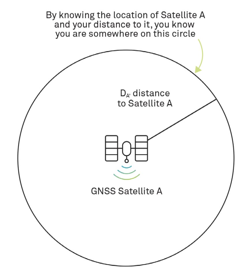
To help us understand trilateration, we’ll present the technique in two dimensions. The receiver calculates its range to Satellite A. As we mentioned, it does this by determining the amount of time it took for the signal from Satellite A to arrive at the receiver and multiplying this time by the speed of light. Satellite A communicated its location (determined from the satellite orbit ephemerides and time) to the receiver, so the receiver knows it is somewhere on a circle with a radius equal to the range and centred at the location of Satellite A, as illustrated in Figure 20. In three dimensions, we would show ranges as spheres, not circles.

The receiver also determines its range to a second satellite, Satellite B. Now the receiver knows it is at the intersection of two circles, at either Position 1 or 2, as shown in Figure 21.

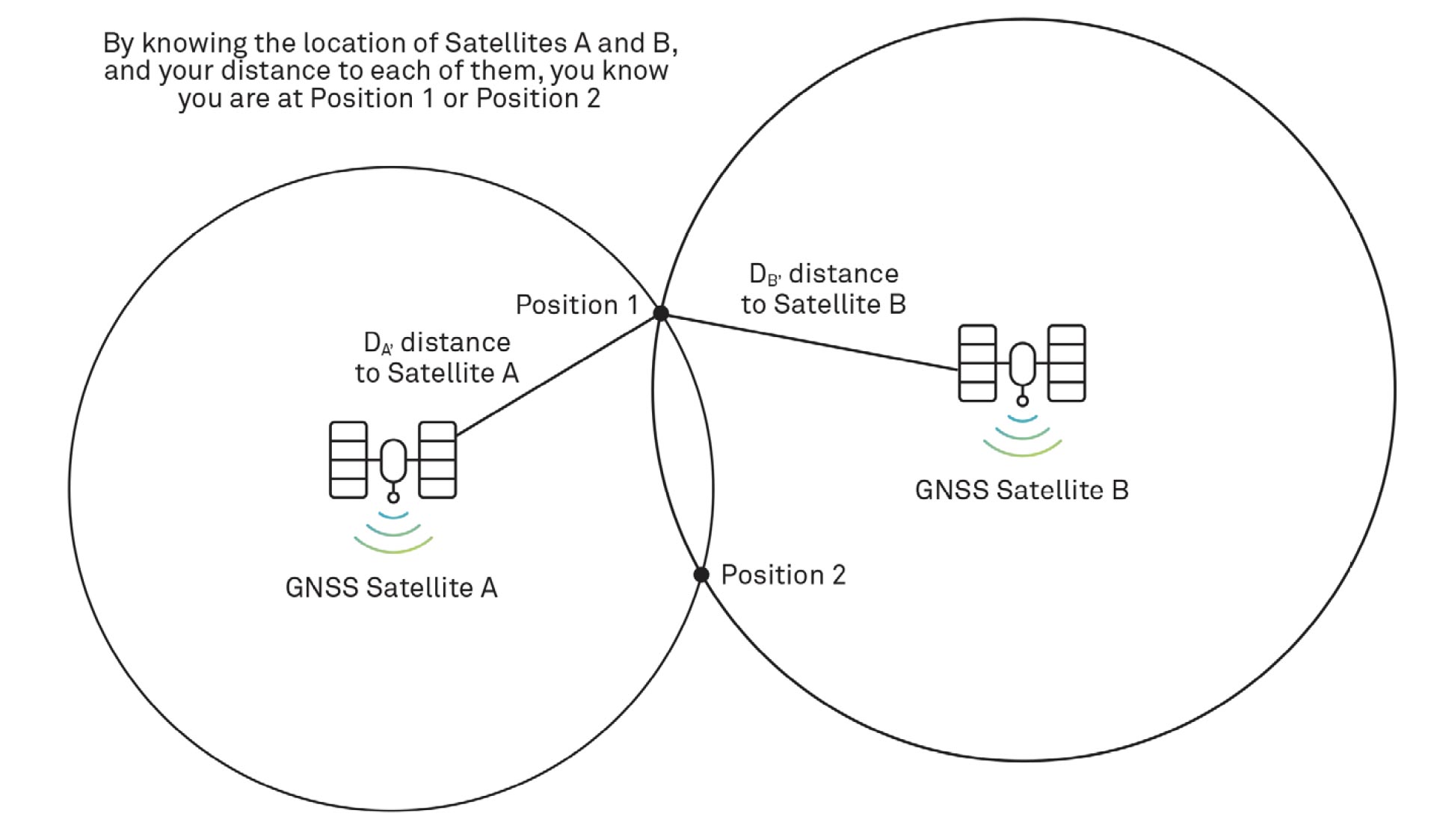
You may be tempted to conclude that ranging to a third satellite would be required to resolve your location to Position 1 or Position 2. However, one of the positions can most often be eliminated as not feasible because, for example, it is in space or in the middle of the Earth. You might also be tempted to extend our illustration to three dimensions and suggest that only three ranges are needed for positioning but four ranges are actually necessary. Why is this?

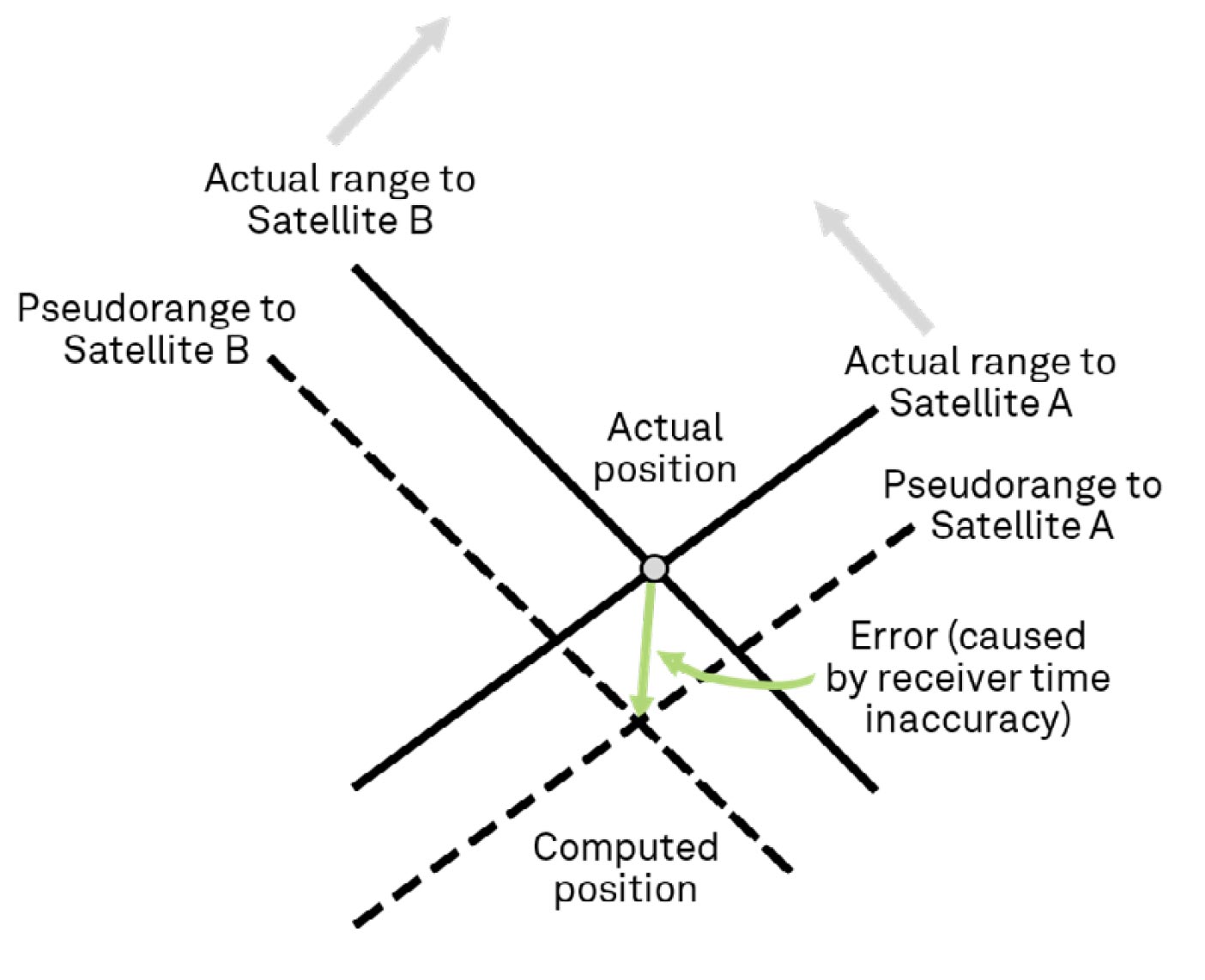
It turns out that receiver clocks are not nearly as accurate as the clocks onboard the satellites. Most are based on quartz crystals. Remember, we said these clocks were accurate to only about five parts per million. If we multiply this by the speed of light, it results in an accuracy of ±1,500 metres (1,640 yards). When we determine the range to two satellites, our computed position, will be out by an amount proportional to the inaccuracy in our receiver clock, as illustrated in Figure 22.

We want to determine our actual position but, as shown in Figure 22, the receiver time inaccuracy causes range errors that result in position errors. The receiver knows there is an error; it just doesn’t know the size of the error. If we now compute the range to a third satellite, it doesn’t intersect the computed position, as shown in Figure 23.

Now for one of the ingenious techniques used in GNSS positioning.

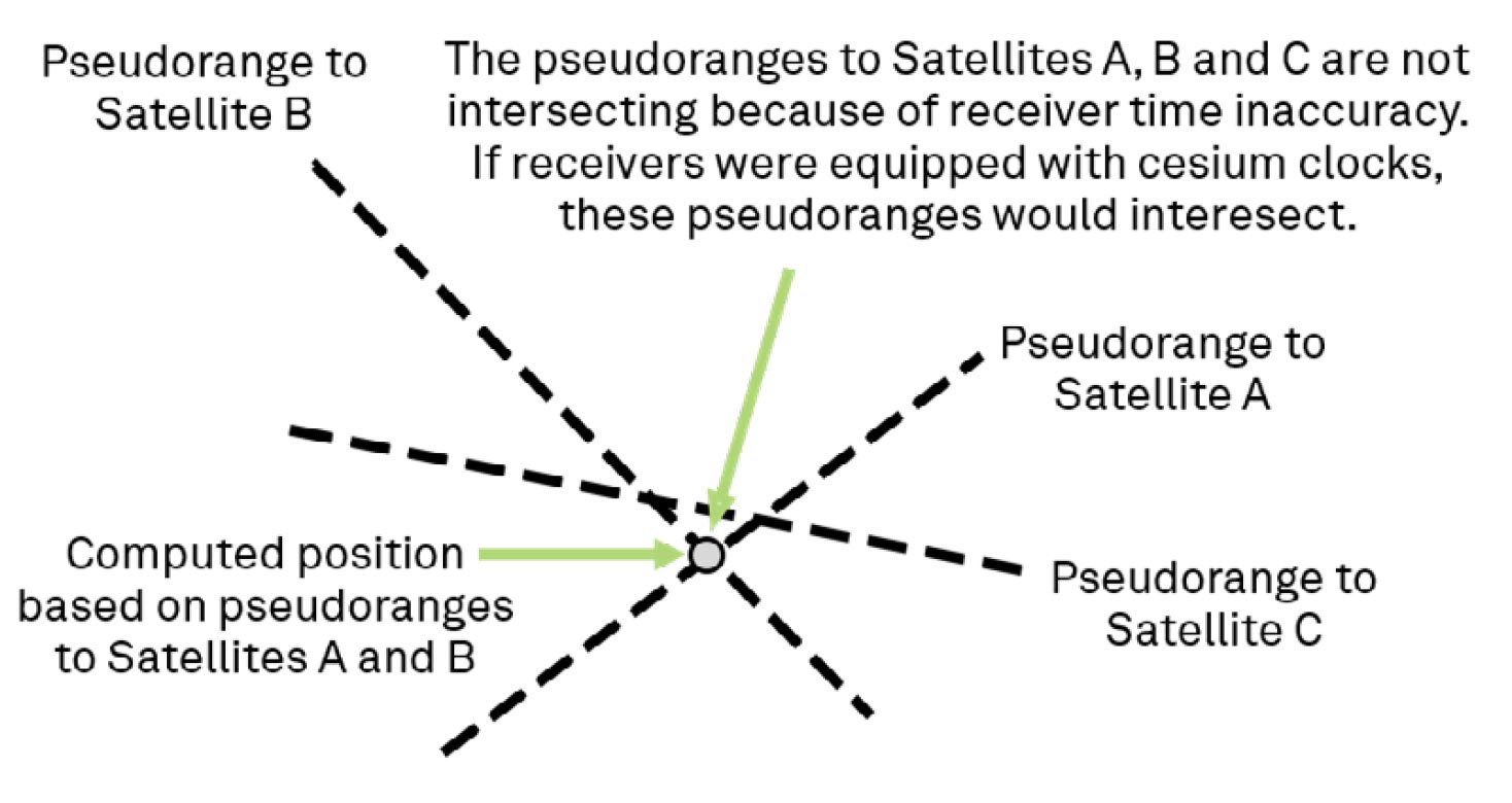
The receiver knows the reason the pseudoranges to the three satellites are not intersecting is because its clock is not very good. The receiver is programmed to advance or delay its clock until the pseudoranges to the three satellites converge at a single point, as shown in Figure 24.

The incredible accuracy of the satellite clock has been “transferred” to the receiver clock, greatly reducing the receiver clock error in the position determination. The receiver now has both an accurate position and extremely accurate time. This presents opportunities for a broad range of applications, as we’ll discuss.

The above technique shows how, in a twodimensional representation, receiver time inaccuracy can be almost eliminated and position determined using ranges to three satellites. When we extend this technique to three dimensions, we need to add a range to a fourth satellite. This is the reason why line-of-sight to a minimum of four GNSS satellites is needed to determine position.

GNSS error sources

A GNSS receiver calculates position based on data received from satellites. However, there are many sources of errors that, if left uncorrected, cause the position calculation to be inaccurate.

The type of error and how it is mitigated is essential to calculating precise position, as the level of precision is only useful to the extent that the measurement can be trusted. This book dedicates three chapters to this important topic. Chapter 4 presents key sources of GNSS errors while Chapter 5 discusses methods of error resolution and impact on accuracy and other performance factors. Chapter 9 presents the equipment and network infrastructure necessary to generate and receive correction data.

Dilution of precision (DOP)

The geometric arrangement of satellites, as they are presented to the receiver, affects the accuracy of position and time calculations. Receivers are ideally designed to use signals from all available satellites in a manner that minimises this so-called “dilution of precision.”

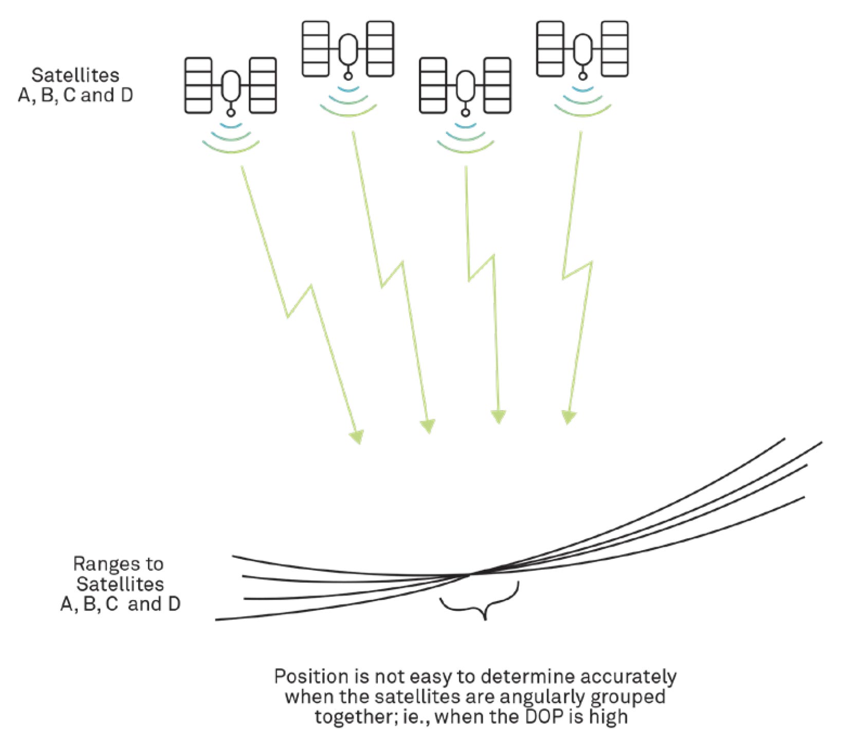
To illustrate DOP, consider the example shown in Figure 25, where the satellites being tracked are clustered in a small region of the sky. As you can see, it is difficult to determine where the ranges intersect. The position is “spread” over the area of range intersections, which is enlarged by range inaccuracies (this can be viewed as a “thickening” of the range lines).

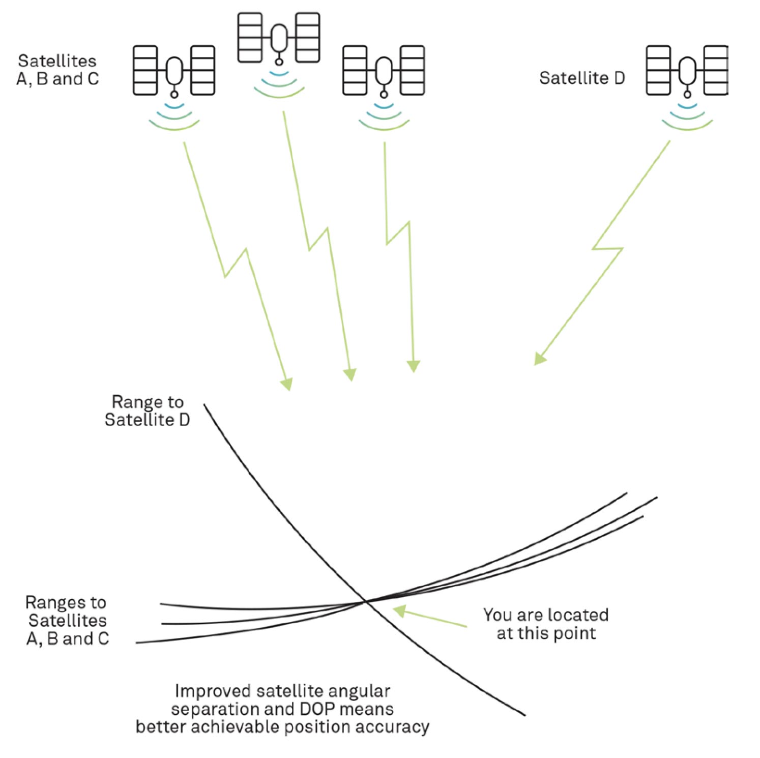
As shown in Figure 26, the addition of a range measurement to a satellite that is angularly separated from the cluster allows the receiver to determine position more precisely.

Although DOP is calculated using complex statistical methods, we can say the following: DOP is a numerical representation of satellite geometry and is dependent on the locations of satellites visible to the receiver.

The smaller the value of DOP, the more precise the time or position calculation. The relationship is shown in the following formula:

Inaccuracy of Computed Position = DOP × Inaccuracy of Range Measurement

So, if DOP is very high, the inaccuracy of the computed position will be much larger than the inaccuracy of the range measurement.

• A DOP above six results in generally unacceptable accuracies for Differential (D) GNSS and RTK operations
• DOP varies with time of day and geographic location
• DOP can be calculated without determining the range. All that is needed is the satellite positions and the approximate receiver location
• Adding more satellites causes the DOP to decrease

DOP can be expressed as a number of separate elements that define the DOP for a particular type of measurement, for example, HDOP (Horizontal Dilution of Precision), VDOP (Vertical Dilution of Precision), and PDOP (Position Dilution of Precision). These factors are mathematically related. In some cases, for example, when satellites are low in the sky, HDOP is low, and it will therefore be possible to get a good to excellent determination of horizontal position (latitude and longitude), but VDOP may only be adequate for a moderate altitude determination.

In Canada and in other countries at high latitudes, GNSS satellites are lower in the sky, so achieving optimal DOP for some applications, particularly where good VDOP is required, can be a challenge.

Applications where the available satellites are low on the horizon or angularly clustered, such as those in urban environments or in deep open-pit mining, may expose users to the pitfalls of DOP.

Chapter 2: Basic GNSS concepts